
What’s All the Fuss About Features?
Features are interesting aspects or attributes of a thing. When we read a feature story, it’s what the news room feels will be the most interesting, compelling story that draws in viewers. Similarly, when we look at a picture, or a Youtube thumbnail, various aspects of that photo or video tend to draw us in. Over the years (thousands of years), humans have gotten pretty good at picking up visual cues. Our ancestors had to stay away from danger, protect their caves from enemies, detect good and bad intentions from the quiver of a lip, and read all sorts of body language form gestures and dances.
Nowadays, it’s not much different, except that we’re teaching computers to pick up on some of the same cues. In computer vision, features are attributes within an image or video that we’d like to isolate as important. A feature could be the mouth, nose, ears, legs, or feet of a face, the corners of a portrait, the roof of a house, or the cap of a bottle.
It is an interesting area, and a grayscale pixel that makes up just a tiny portion of an entire photograph won’t tell us much. Instead, a collection of these pixels within a given area of interest is what we’re after. If an image can be processed, then certainly we can isolate areas of that photo for further inspection, and match it with like or exact objects – and that is what we’re going to explore.
Types of Detection
We all should know the power that OpenCV brings to the table, and it does not fall short with its methods of feature detection. There is Harris corner detection, Shi-Tomasi corner detection, Scale-Invariant Feature transform (SIFT), and Speeded-Up Robust Features (SURF), to name a few. Harris and Shi-Tomasi both have different ways of detecting corners, and using one over the other comes down mostly to personal preference. Use them and find as many boxes and portraits in images and videos as you like, but we’re looking for the big power brokers. We’re gonna use SIFT in this example, and SURF works great too, but not today my friends.
Both SURF and SIFT work by detecting points of interest, and then forming a descriptor of said points. If you’d like the technical explanation of SIFT, take a look at the source. The explanation goes into depth about how this type of feature detection and matching has enough robustness to handle changing light conditions, orientations, angles, etc. Pretty, pretty…pret-tyyy good stuff.
Basics
The basic workflow we’ll be using is to take an image, automatically detect features which would make this object unique from similar objects, attempt to describe those features, and then compare those unique features (if any are found) with another image or video that contains the original image/video, perhaps in a group to make it more challenging. Imagine, if we keyed a particular make and model of a car, setup a camera, and waited to see if and when that car showed up in front of our house again. You could setup a network of cameras to look for a missing person, or key an image of a lost bike for cameras around a college campus. Just make sure you do so within the laws of your jurisdiction, of course.
The bulk of the work for matching keyed features is handled by a version of the unsupervised clustering classifier, the k-Nearest Neighbor (kNN) algorithm. In our example, we train a kNN model to detect descriptors from our original training image, and then use a query set to see if we find matches.
Code Exploration and Download Resources
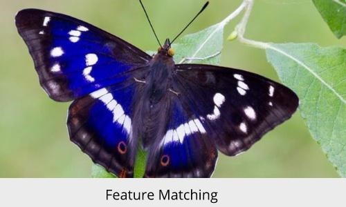
Here’s our original image to start with. That butterfly is known as the Purple Emperor, and it is beautiful, oh yes. And it also feeds on rotting flesh. Be an admirer when you’re combing the British countryside, but not too close. Full code and resources can be downloaded here.

Use Python 3 if you can, an installation of OpenCV (3+ if possible), and the usual Numpy and Matplotlib. It may be necessary to install along with OpenCV, opencv-contrib. In my case using Python 3+, I had installed OpenCV though Homebrew on a Mac/Linux install, and had to find an alternative way to invoke the SIFT command:
import cv2

import matplotlib.pyplot as plt

import numpy as np

n_kp = 100 #limit the number of possible matches

# Initiate SIFT detector

#sift = cv2.SIFT() #in Python 2.7 or earlier?

sift = cv2.xfeatures2d.SIFT_create(n_kp)
If you still have trouble getting your interpreter to recognize SIFT, try using the Python command line or terminal, and invoking this function:
>>help(cv2.xfeatures2d)
Then exit and run these lines to see if everything checks out:
>>import cv2

>>>image = cv2.imread("any_test_image.jpg")

>>>sift = cv2.xfeatures2d.SIFT_create()

>>>(kps, descs) = sift.detectAndCompute(gray, None)

>>>print("# kps: {}, descriptors: {}".format(len(kps), des

cs.shape))
If you get a response, and not an error message, you’re all set. I’ve set the number of possible feature matches to 100 with the variable n_kp , if only to make our final rendition more visually pleasing. Try it without this parameter – it’s ugly, but gives you a sense of all the features that match; some are more accurate than others.
MIN_MATCHES = 10

img1 = cv2.imread('butterfly_orig.png',0) # queryImage

img2 = cv2.imread('butterflies_all.png',0) # trainImage

# find the keypoints and descriptors with SIFT

keyp1, desc1 = sift.detectAndCompute(img1,None)

keyp2, desc2 = sift.detectAndCompute(img2,None)

FLANN_INDEX_KDTREE = 0

src_params = dict(checks = 50)

idx_params = dict(algorithm = FLANN_INDEX_KDTREE, trees =

5)
With our training and test images set, we send SIFT off of detect features. We set MIN_MATCHES to 10, meaning that we’ll need at least 10 of the 100 max possible matches to be detected for us to accept them as identifiable features. Making use of the Fast Library for Approximate Nearest Neighbors (FLANN) classifier, we now want to actually search for recognizable patterns between our original training set and our target image. First, we’ve set up index idx_params , and search src_params , and we’ll run the method FlannBasedMatcher to perform a quick search to determine matches.
flann = cv2.FlannBasedMatcher(idx_params, src_params)

matches = flann.knnMatch(desc1,desc2,k=2)

# only good matches using Lowe's ratio test

good_matches = []

for m,n in matches:

if m.distance < 0.7*n.distance:

#good_matches = filter(lambda x: x[0].distance<0.7

*x[1].distance,m)

good_matches.append(m)
We’ve also saved to matches , a run of descriptors from both images to see if they match. From flann.knnMatch will come up with a list of commonalities between the two sets of descriptors. Keep in mind that the more matches that are found between the training and query (target image) set, the more likely that our training pattern has been found in our target image. Of course, not all features will accurately line up. We used k=2 for our k parameter, and that means the algorithm is searching for the two closest descriptors for each match.
Invariably, one of these two matches will be further away from the correct match, so to filter out the worst matches, and filter in the best ones, we’ve setup a list and a loop to catch the good_matches . By using the Lowe’s ratio test, a good match comes along when ratio of distances between the first and second match is less than a certain number – in this case 0.7.
We’ve now found our best-matching keypoints, if there are any, and now we have to iterate over them, and do fun stuff like draw circles and lines between key points so we won’t be confused at what we’re looking at.
if len(good_matches)>MIN_MATCHES:

src_pts = np.float32([ keyp1[m.queryIdx].pt for m in g

ood_matches ]).reshape(-1,1,2)

train_pts = np.float32([ keyp2[m.trainIdx].pt for m in

good_matches ]).reshape(-1,1,2)

M, mask = cv2.findHomography(src_pts, train_pts, cv2.R

ANSAC,5.0)

matchesMask = mask.ravel().tolist()

h,w = img1.shape

pts = np.float32([ [0,0],[0,h-1],[w-1,h-1],[w-1,0] ]).

reshape(-1,1,2)

dst = cv2.perspectiveTransform(pts,M)

img2 = cv2.polylines(img2,[np.int32(dst)],True,255,3,

cv2.LINE_AA)

else:

print("Not enough matches have been found - {}/{}".for

mat(len(good_matches),MIN_MATCHES))

matchesMask = None

draw_params = dict(matchColor = (0,0,255), singlePointColo

r = None,matchesMask = matchesMask,flags = 2)

img3 = cv2.drawMatches(img1,keyp1,img2,keyp2,good_matches,

None,**draw_params)

plt.imshow(img3, 'gray'),plt.show()
We store src_pts and train_pts , where each match, m , is a store of the index of keypoint lists. m.queryIdx refers to the index of query key points, and m.trainIdx refers to the index of the training key points in the keyp2 list. So, our lists and matching key points are saved, but what’s this cv2.findHomography ? This method makes our matching more robust, by finding the homography transformation matrix between the feature points. Thus, if our target image is distorted or has a different perspective transformation from the camera or otherwise, we can bring the desired feature points into the right plane as our training image.
RANSAC stands for Random Sample Consensus, and it involves some heavy lifting whereby the training image is used to determine where those same, matching features might be in the new image that may have been twisted, tilted, warped, or otherwise transformed. The best matches after any transforms are known as inliers, and those that didn’t make the cut are called outliers. Again, if you take a moment to think about that, the power of feature detection after significant transforms is pretty interesting…maybe a bit too interesting.
We then draw lines to match the original image key points with the query transforms, and the output might look something like this:

I’m calling this the butterfly effect.
Takeaways
It’s not as if you needed another example, but OpenCV’s computer vision is a powerful tool. We grabbed an image, classified its unique features, then partially obstructed that image in a busier query image, only to find that our feature detection was so strong that it had no problem whatsoever finding and matching the features and descriptors from our target image. The applications of this technology are being implemented today, and if you explore it now, you’ll be well on your way to creating something for tomorrow.